The four dc motors used to build the structure are controlled by microcontroller Atmel 89C51.

1 AT89C51 from Atmel Corporation:

The AT89C51 is a low-power, high-performance CMOS 8-bit microcomputer with 4K
bytes of Flash programmable and erasable read only memory (PEROM). The device
is manufactured using Atmel’s high-density nonvolatile memory technology and is
compatible with the industry-standard MCS-51 instruction set and pinout. The on-chip
Flash allows the program memory to be reprogrammed in-system or by a conven-
tional nonvolatile memory programmer. By combining a versatile 8-bit CPU with Flash
on a monolithic chip, the Atmel AT89C51 is a powerful microcomputer which provides
a highly-flexible and cost-effective solution to many embedded control applications.
The AT89C51 provides the following standard features: 4K bytes of Flash, 128 bytes of RAM, 32 I/O lines, two 16-bit timer/counters, a five vector two-level interrupt architecture, a full duplex serial port, on-chip oscillator and clock circuitry. In addition, the AT89C51 is designed with static logic for operation down to zero frequency and supports two software selectable power saving modes. The Idle Mode stops the CPU while allowing the RAM, timer/counters, serial port and interrupt system to continue functioning. The Power-down Mode saves the RAM contents but freezes the oscillator disabling all other chip functions until the next hardware reset.


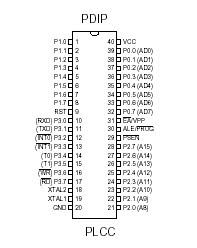
2 Pin configuration:





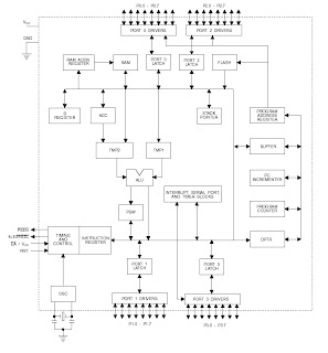
3 Block diagram


4 Pin Description

VCC
Supply voltage.

GND
Ground.

Port 0
Port 0 is an 8-bit open-drain bi-directional I/O port. As an output port, each pin can sink eight TTL inputs. When 1s are written to port 0 pins, the pins can be used as high-impedance inputs.
Port 0 may also be configured to be the multiplexed low-order address/data bus during accesses to external program and data memory. In this mode P0 has internal pullups. Port 0 also receives the code bytes during Flash programming, and outputs the code bytes during program verification. External pullups are required during program verification.

Port 1
Port 1 is an 8-bit bi-directional I/O port with internal pullups. The Port 1 output buffers can sink/source four TTL inputs. When 1s are written to Port 1 pins they are pulled high by the internal pullups and can be used as inputs. As inputs, Port 1 pins that are externally being pulled low will source current (IIL) because of the internal pullups. Port 1 also receives the low-order address bytes during Flash programming and verification.

Port 2
Port 2 is an 8-bit bi-directional I/O port with internal pullups. The Port 2 output buffers can sink/source four TTL inputs. When 1s are written to Port 2 pins they are pulled high by
the internal pullups and can be used as inputs. As inputs, Port 2 pins that are externally being pulled low will source current (IIL) because of the internal pullups. Port 2 emits the high-order address byte during fetches from external program memory and during accesses to external data memory that use 16-bit addresses (MOVX @ DPTR). In this application, it uses strong internal pullups when emitting 1s. During accesses to external data memory that use 8-bit addresses (MOVX @ RI), Port 2 emits the contents of the P2 Special Function Register.
Port 2 also receives the high-order address bits and some control signals during Flash programming and verification.

Port 3
Port 3 is an 8-bit bi-directional I/O port with internal pullups. The Port 3 output buffers can sink/source four TTL inputs. When 1s are written to Port 3 pins they are pulled high by the internal pullups and can be used as inputs. As inputs, Port 3 pins that are externally being pulled low will source current (IIL) because of the pullups.

RST
Reset input. A high on this pin for two machine cycles while the oscillator is running resets the device.

XTAL1
Input to the inverting oscillator amplifier and input to the internal clock operating circuit.



XTAL2
Output from the inverting oscillator amplifier.

Oscillator Characteristics
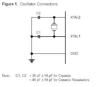
XTAL1 and XTAL2 are the input and output, respectively, of an inverting amplifier which can be configured for use as an on-chip oscillator, as shown in Figure 1. Either a quartz crystal or ceramic resonator may be used. To drive the device from an external clock source, XTAL2 should be left unconnected while XTAL1 is driven as shown in Figure 2. There are no requirements on the duty cycle of the external clock signal, since the input to the internal clocking circuitry is through a divide-by-two flip-flop, but minimum and maximum voltage high and low time specifications must be observed.
Idle Mode
In idle mode, the CPU puts itself to sleep while all the on-chip peripherals remain active. The mode is invoked by software. The content of the on-chip RAM and all the special functions registers remain unchanged during this mode. The idle mode can be terminated by any enabled interrupt or by a hardware reset.
It should be noted that when idle is terminated by a hardware reset, the device normally resumes program execution, from where it left off, up to two machine cycles before the internal reset algorithm takes control. On-chip hardware inhibits access to internal RAM in this event, but access to the port pins is not inhibited. To eliminate the possibility of an unexpected write to a port pin when Idle is terminated by reset, the instruction following the one that invokes Idle should not be one that writes to a port pin or to external memory.



5 Design of dc drive

5.1 Block diagram:




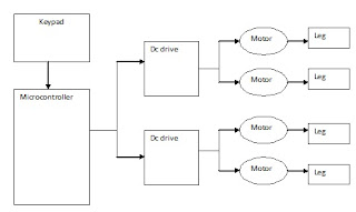
5.2 Block diagram of dc drive

5.3 Description of components used

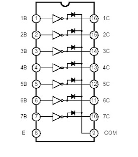
Uln2003

DESCRIPTION

The ULN2003 is a monolithic high voltage and high current Darlington transistor arrays. It consists of seven NPN darlington pairs that features high-voltage outputs with common cathode clamp diode for switching inductive loads. The collector-current rating of a single darlington pair is 500mA. The darlington pairs may be paralleled for higher current capability. Applications include relay drivers, hammer drivers, lamp drivers, display drivers (LED gas discharge), line drivers, and logic buffers.

FEATURES
• 500mA rated collector current(Single output)
• High-voltage outputs: 50V
• Inputs compatibale with various types of logic.
• Relay driver application


Logic Diagram

Face Detection and make ROI Code in C - opencv

#include "stdafx.h"
#ifndef _EiC
#include "cv.h"
#include "highgui.h"
#include
#include
#include
#include
#include
#include
#include
#include
#include
#endif
#ifdef _EiC
#define WIN32
#endif

static CvMemStorage* storage = 0;
static CvHaarClassifierCascade* cascade = 0;
void detect_and_draw( IplImage* image, int );
const char* cascade_name ="haarcascade_frontalface_default.xml";
int main( int argc, char** argv )
{
CvCapture* capture = 0;
IplImage *frame, *frame_copy = 0;
int counter=0;
int optlen = strlen("--cascade= ");
const char* input_name;
cascade =(CvHaarClassifierCascade*)cvLoad( "haarcascade_frontalface_default.xml",0, 0, 0 );
if( !cascade )
{
fprintf( stderr, "ERROR: Could not load classifier cascade\n" );
return -1;
}
storage = cvCreateMemStorage( 0);
capture = cvCaptureFromCAM( 0 );
cvNamedWindow( "result", 1 );
if( capture )
{
for(;;)
{

if( !cvGrabFrame( capture ))
break;
frame = cvRetrieveFrame( capture );
if( !frame )
break;
if( !frame_copy )
frame_copy = cvCreateImage( cvSize(frame->width,frame->height),
IPL_DEPTH_8U, frame->nChannels );

if( frame->origin == IPL_ORIGIN_TL )
cvCopy( frame, frame_copy, 0 );
else
cvFlip( frame, frame_copy, 0 );
++counter;
cvSaveImage("F.jpg", frame_copy);
detect_and_draw( frame_copy,counter);

if( cvWaitKey( 10 ) >= 0 )
break;

}

cvReleaseImage( &frame_copy );
cvReleaseCapture( &capture );
}


return 0;
}

void detect_and_draw( IplImage* img, int counter)
{
int scale = 1;
IplImage* temp = cvCreateImage(
cvSize(img-> width/scale, img->height/ scale), 8, 3 );
CvPoint pt1, pt2;
IplImage* face = 0;
int i;
cvClearMemStorage( storage );
if( cascade )
{
CvSeq* faces = cvHaarDetectObjects ( img, cascade, storage,1.1, 2, CV_HAAR_DO_CANNY_PRUNING,cvSize(40, 40) );
for( i = 0; i < (faces ? faces->total : 0); i++ )
{
CvRect* r = (CvRect*)cvGetSeqElem( faces, i );
pt1.x = r->x*scale;
pt2.x = (r->x+r->width) *scale;
int width = pt2.x-pt1.x;
pt1.y = r->y*scale;
pt2.y = (r->y+r->height) *scale;
int height = pt2.y-pt1.y;

cvRectangle( img, pt1, pt2, CV_RGB(255,0, 0), 1, 8, 0 );

if(counter==1)
{
cvSetImageROI(img, cvRect(pt1.x+1,pt1.y+1,width-1,height-1));
cvSaveImage("Roi.jpg",img);
cvResetImageROI(img);
}



}
}

cvShowImage( "result", img );
cvReleaseImage( &temp );
}

#ifdef _EiC
main(1,"facedetect. c");
#endif

Principal Component Analysis matlab code

The Principal Component Analysis (PCA) is one of the most successful techniques that have been used in image recognition and compression. PCA is a statistical method under the broad title of factor analysis. The purpose of PCA is to reduce the large dimensionality of the data space (observed variables) to the smaller intrinsic dimensionality of feature space (independent variables), which are needed to describe the data economically. This is the case when there is a strong correlation between observed variables.

The jobs which PCA can do are prediction, redundancy removal, feature extraction, data compression, etc. Because PCA is a classical technique which can do something in the linear domain, applications having linear models are suitable, such as signal processing, image processing, system and control theory, communications, etc



WHEN PUBLISHING A PAPER AS A RESULT OF RESEARCH CONDUCTED BY USING THIS CODE
OR ANY PART OF IT, MAKE A REFERENCE TO THE FOLLOWING PAPER:
Delac K., Grgic M., Grgic S., Independent Comparative Study of PCA, ICA, and LDA
on the FERET Data Set, International Journal of Imaging Systems and Technology,
Vol. 15, Issue 5, 2006, pp. 252-260

=====================================================================================

pca.m

-------------------------------------------------------------------------------------

function pca (path, trainList, subDim)

if nargin < 3
subDim = dim - 1;
end;

disp(' ')

load listAll;

% Constants
numIm = 3816;


% Memory allocation for DATA matrix
fprintf('Creating DATA matrix\n')
tmp = imread ( [path char(listAll(1)) '.pgm'] );
[m, n] = size (tmp); % image size - used later also!!!
DATA = uint8 (zeros(m*n, numIm)); % Memory allocated
clear str tmp;

% Creating DATA matrix
for i = 1 : numIm
im = imread ( [path char(listAll(i)) '.pgm'] );
DATA(:, i) = reshape (im, m*n, 1);
end;
save DATA DATA;
clear im;

% Creating training images space
fprintf('Creating training images space\n')
dim = length (trainList);
imSpace = zeros (m*n, dim);
for i = 1 : dim
index = strmatch (trainList(i), listAll);
imSpace(:, i) = DATA(:, index);
end;
save imSpace imSpace;
clear DATA;

% Calculating mean face from training images
fprintf('Zero mean\n')
psi = mean(double(imSpace'))';
save psi psi;

% Zero mean
zeroMeanSpace = zeros(size(imSpace));
for i = 1 : dim
zeroMeanSpace(:, i) = double(imSpace(:, i)) - psi;
end;
save zeroMeanSpace zeroMeanSpace;
clear imSpace;

% PCA
fprintf('PCA\n')
L = zeroMeanSpace' * zeroMeanSpace; % Turk-Pentland trick (part 1)
[eigVecs, eigVals] = eig(L);

diagonal = diag(eigVals);
[diagonal, index] = sort(diagonal);
index = flipud(index);

pcaEigVals = zeros(size(eigVals));
for i = 1 : size(eigVals, 1)
pcaEigVals(i, i) = eigVals(index(i), index(i));
pcaEigVecs(:, i) = eigVecs(:, index(i));
end;

pcaEigVals = diag(pcaEigVals);
pcaEigVals = pcaEigVals / (dim-1);
pcaEigVals = pcaEigVals(1 : subDim); % Retaining only the largest subDim ones

pcaEigVecs = zeroMeanSpace * pcaEigVecs; % Turk-Pentland trick (part 2)

save pcaEigVals pcaEigVals;

% Normalisation to unit length
fprintf('Normalising\n')
for i = 1 : dim
pcaEigVecs(:, i) = pcaEigVecs(:, i) / norm(pcaEigVecs(:, i));
end;

% Dimensionality reduction.
fprintf('Creating lower dimensional subspace\n')
w = pcaEigVecs(:, 1:subDim);
save w w;
clear w;

% Subtract mean face from all images
load DATA;
load psi;
zeroMeanDATA = zeros(size(DATA));
for i = 1 : size(DATA, 2)
zeroMeanDATA(:, i) = double(DATA(:, i)) - psi;
end;
clear psi;
clear DATA;

% Project all images onto a new lower dimensional subspace (w)
fprintf('Projecting all images onto a new lower dimensional subspace\n')
load w;
pcaProj = w' * zeroMeanDATA;
clear w;
clear zeroMeanDATA;
save pcaProj pcaProj;

=====================================================================================

createDistMat.m

-------------------------------------------------------------------------------------

function distMat = createDistMat (proj, metric)

% Memory allocation
distMat = zeros(max(size(proj)));

switch (metric)

case 'L1'
distMat = pdist(proj', 'cityblock');
case 'L2'
distMat = pdist(proj', 'euclidean');
case 'COS'
distMat = pdist(proj', 'cosine');

otherwise
error('%s metric not supported.', metric);

end; % switch (metric) ends here

distMat = squareform(distMat);

=====================================================================================

feret.m

-------------------------------------------------------------------------------------

function [FERET] = feret(distMat, rank)

% Load feretGallery and probe lists
load listAll;
load feretGallery;
load fb;
load fc;
load dup1;
load dup2;

% Constants (number of images in feretGallery and probes)
numGalleryImgs = size (feretGallery, 1);
numFbImgs = size (fb, 1);
numFcImgs = size (fc, 1);
numDup1Imgs = size (dup1, 1);
numDup2Imgs = size (dup2, 1);

% Get the list of positions where feretGallery images are located in the list
% of all images and store it in variable index
feretGalleryIndex = getIndex (feretGallery, listAll);

% Get the list of all the probe images
fbIndex = getIndex (fb, listAll);
fcIndex = getIndex (fc, listAll);
dup1Index = getIndex (dup1, listAll);
dup2Index = getIndex (dup2, listAll);

% Calculate ranks for the CMS curve
% The results are stores in a structure
FERET.fb = getResults (distMat, feretGallery, feretGalleryIndex, fb, fbIndex, numFbImgs, rank);
FERET.fc = getResults (distMat, feretGallery, feretGalleryIndex, fc, fcIndex, numFcImgs, rank);
FERET.dup1 = getResults (distMat, feretGallery, feretGalleryIndex, dup1, dup1Index, numDup1Imgs, rank);
FERET.dup2 = getResults (distMat, feretGallery, feretGalleryIndex, dup2, dup2Index, numDup2Imgs, rank);

%**************************************************************************
% Statistics (CMS curve, total number of probe images)
%**************************************************************************

function [RESULTS] = getResults (distMat, feretGallery, feretGalleryIndex, probe, probeIndex, numProbeImgs, rank)

for j = 1 : rank
for i = 1 : numProbeImgs

position = probeIndex(i);
currentRow = distMat(position,:);
reduced = currentRow(1, feretGalleryIndex);

[Y, I] = sort(reduced);
inx = I(j);

% Determine if G=H based on the first 5 characters of the filename
G = char(feretGallery(inx));
H = char(probe(i));
correct(i) = strncmp(G, H, 5);
% if G=H correct(i)=1, else 0

end;

% Rank 1 result (percentage)
if j == 1
RESULTS.rank1 = (sum(correct)/numProbeImgs)*100;
end;

% Percentage of correctly recognized images for a given probe set
RESULTS.perc(j) = (sum(correct)/numProbeImgs)*100;

% CMS curve
RESULTS.cms(j) = sum(RESULTS.perc(1:j));

end;

% Total number of probe images
RESULTS.numProbeImgs = numProbeImgs;
%**************************************************************************

%**************************************************************************
% Find positions of probe or feretGallery images in the list of all images
%**************************************************************************

function [index] = getIndex (sub, all)

num = size (sub, 1);
for i = 1 : num
index(i) = strmatch(sub(i), all);
end;
%**************************************************************************

Viola-Jones object detection framework

The Viola-Jones object detection framework is the first object detection framework to provide competitive object detection rates in real-time proposed in 2001 by Paul Viola and Michael Jones.

Introduction
Object detection is detecting a specified object class such as cars, faces, plates ext. in a given image or a video sequence. Object detection has many applications in computer based vision such as object tracking, object recognition, and scene surveillance.

The technique relies on the use of simple Haar-like features that are evaluated quickly through the use of a new image representation. Based on the concept of an “Integral Image” it generates a large set of features and uses the boosting algorithm AdaBoost to reduce the over-complete set and the introduction of a degenerative tree of the boosted classifiers provides for robust and fast interferences. The detector is applied in a scanning fashion and used on gray-scale images, the scanned window that is applied can also be scaled, as well as the features evaluated.

In the technique only simple rectangular (Haar-like) features are used, reminiscent to Haar basis functions. These features are equivalent to intensity difference readings and are quite easy to compute. There are three feature types used with varying numbers of sub-rectangles, two, two rectangles, one three and one four rectangle feature types. Using rectangular features instead of the pixels in an image provides a number of benefits, namely a sort of a ad-hoc domain knowledge is implied as well as a speed increase over pixel based systems. The calculation of the features is facilitated with the use of an “integral image”. With the introduction of a integral image Viola and Jones are able to calculate in one pass of the sample image, and is one of the keys to the speed of the system. An integral image is similar to a “summed are table”, used in computer graphics but its use is applied in pixel area evaluation.

It was outlined that the implementation of a system that used such features would provide a feature set that was far too large, hence the feature set must be only restricted to a small number of critical features. This is done with the use of boosting algorithm, AdaBoost. Interference is enhanced with the use of AdaBoost where a small set of features is selected from a large set, and in doing so a strong hypothesis is formed, in this case resulting in a strong classifier. Simply having a reduced set of features was not enough to reduce the vast amounts of computation in a detector task, since it is naturally a probabilistic one, hence Viola and Jones proposed the use of degenerative tree of classifiers.

Described by Viola and Jones as a degenerative tree, and sometimes referred to as a decision stump, its use also speeds the detection process. A degenerative tree is the daisy chaining of general to specific classifiers, whereby the first few classifiers are general enough to discount an image sub window and so on the time of further observations by the more specific classifiers down the chain, this can save a large degree of computation.

Integral Image
In order to be successful a face detection algorithm must possess two key features, accuracy and speed. There is generally a trade-off between the two. Through the use of a new image representation, termed integral images, Viola and Jones describe a means for fast feature evaluation, and this proves to be an effective means to speed up the classification task of the system.

Integral images are easy to understand, they are constructed by simply taking the sum of the luminance values above and to the left of a pixel in an image. Viola and Jones make note of the fact that the integral image is effectively the double integral of the sample image, first along the rows then along the columns. Integral images are equivalent to summed-area tables, yet their use is not texture mapping, being so, their implementation us quite well documented.

1 1 1
1 1 1
1 1 1


1 2 3
2 4 6
3 6 9
The brilliance in using an integral image to speed up a feature extraction lies in the fact that any rectangle in an image can be calculated from that images integral image, in only four indexes to the integral image. This makes the otherwise exhaustive process of summing luminances quite rapid. In fact the calculation of an images integral image can be calculated in only one pass of the image, and Matlab experiments have shown that a large set of images (12000) can be calculated within less than 2 seconds.

Integral application
Given a rectangle specified as four coordinates A(x1,y1) upper left and D(x4,y4) lower right, evaluating the area of the rectangle is done in four image references to the integral image, this represents a huge performance increase in terms of feature extraction.

Sum of grey rectangle = D - (B + C) + A

Since both rectangle B and C include rectangle A the sum of A has to be added to the calculation.


Source:
http://www.codeproject.com/Articles/85113/Efficient-Face-Detection-Algorithm-using-Viola-Jon.aspx

Robust Face Detection in C/C++ (Haar-like features)

Best solution might be Haar-like features.

Viola and Jones adapted the idea of using Haar wavelets and developed the so called Haar-like features. A Haar-like feature considers adjacent rectangular regions at a specific location in a detection window, sums up the pixel intensities in these regions and calculates the difference between them. This difference is then used to categorize subsections of an image. For example, let us say we have an image database with human faces. It is a common observation that among all faces the region of the eyes is darker than the region of the cheeks. Therefore a common haar feature for face detection is a set of two adjacent rectangles that lie above the eye and the cheek region. The position of these rectangles is defined relative to a detection window that acts like a bounding box to the target object (the face in this case).

source: http://en.wikipedia.org/wiki/Haar-like_features

The Postroom Computer Assignment solution

ADD:

%ADDLL msw1 lsw1 msw2 lsw2

MOV .R1 @&:msw1:
MOV .R0 @&:lsw1:
MOV .R3 @&:msw2:
MOV .R2 @&:lsw2:

ADD .R0 .R2
JMP &CRY :carrye: ;ADD lsw1 and lsw2 and if carry then GOTO carrye

:backy:
ADD .R1 .R3
JMP :outy: ; Add msw1 and msw2 and GOTO show output

:carrye:
ADD .R1 &1 ; Just add 1 the carry of lsw1 and lsw2 addition
JMP :backy: ; Go back to add Msw1 and MSW2

:outy:

OUT .R1 &USGN
MOV .R1 &9 ;initialise digit count
:loop: SHF .R0 &1 ;shift number one place to the left
MOV .R2 .CAR ;copy the carry to R2
ADD .R2 &'0' ;add the ASCII code for 0
OUT .R2 &CHR ;output the digit
SUB .R1 &1 ;decrease digit count
JMP >Z :loop: ;if still digits to print repeat the loop

%


MASK:

%MSKL msw1 lsw1 msw2 lsw2

MOV .R1 @&:msw1:
MOV .R0 @&:lsw1:
MOV .R3 @&:msw2:
MOV .R2 @&:lsw2:

MSK .R1 .R3
MSK .R0 .R2

OUT .R1 &USGN

MOV .R1 &9 ;initialise digit count
:loop: SHF .R0 &1 ;shift number one place to the left
MOV .R2 .CAR ;copy the carry to R2
ADD .R2 &'0' ;add the ASCII code for 0
OUT .R2 &CHR ;output the digit
SUB .R1 &1 ;decrease digit count
JMP >Z :loop: ;if still digits to print repeat the loop

%


SHIFT:

%SHFTL msw1 lsw1 shftamnt

MOV .R1 @&:msw1:
MOV .R0 @&:lsw1:
MOV .R3 @&:shftamnt:


MOV .R9 .R3
MOV .R5 &1
ADD .R5 .R9
JMP >Z :looppos: ; check either we want to go left or right


MOV .R5 &9
:loopneg: ; we got tough task right shift

MOV .R7 .R1
JMP :loopget: ; approch use it shift left 9 times to get the number which we have to transfer from msw to lsw
:loopret:

JMP &:multget: ; multiply tht number with 100000000 and add in the lsw to make proper right shift simple as that
:done:
SHF .R0 @&:amount:
ADD .R0 .R8
SHF .R1 @&:amount:
MOV .R5 &9
ADD .R9 &1
JMP <Z :loopneg: ; wait untill all 9 digits are properly transfered
JMP :outy:

:looppos:
SHF .R1 &1 ;shift number one place to the left
SHF .R0 &1 ;shift number one place to the left
MOV .R2 .CAR ;copy the carry to R2 and place it in the msw by simply adding as msw is already shifted and zero in decimal place
ADD .R1 .R2
SUB .R9 &1
JMP >Z :looppos:
JMP :outy: ; display output


:outy:
OUT .R1 &USGN
MOV .R1 &9 ;initialise digit count
:loop: SHF .R0 &1 ;shift number one place to the left
MOV .R2 .CAR ;copy the carry to R2
ADD .R2 &'0' ;add the ASCII code for 0
OUT .R2 &CHR ;output the digit
SUB .R1 &1 ;decrease digit count
JMP >Z :loop: ;if still digits to print repeat the loop

JMP :endy:


:loopget: ; loop to get the decimal from msw which needs to be transfered in lsw
SHF .R7 &1
MOV .R8 .CAR ; can also be achieved in single 9 shifts
SUB .R5 &1
JMP >Z :loopget:
JMP :loopret:



:multget: ; multiply only by shifting 8 times
SHF .R8 &8
JMP &:done:


:amount: (-1)

:endy:
%


SUB:

%SUBLL msw1 lsw1 msw2 lsw2

MOV .R1 @&:msw1:
MOV .R0 @&:lsw1:
MOV .R3 @&:msw2:
MOV .R2 @&:lsw2:

SUB .R1 .R3 ;sub msw1 msw2
JMP >Z :firstpos: ; if the answer is pos then our net answer is pos as well
JMP &EQZ :firstzer: ; if first answer is zero thn use this jum

SUB .R0 .R2 ; Sub lsw1 lsw2 you will only come here if result of sub msw1 msw2 was neg
JMP >Z :firstnegsecpos: ; Sub lsw1 lsw2 is pos number thn use this
JMP <Z :firstnegsecneg: ; Sub lsw1 lsw2 is neg number thn use this
JMP :outy2:

:firstnegsecneg: ; both individual sub resulted in neg our over all result is neg
MOV .R6 .R0 ; we have to now get our correct result
MOV .R8 &0 ; approch used it just convert the sec neg sub lsw1 lsw2 to pos
:loopy:
ADD .R8 &1
ADD .R6 &1 ; use loop to convert neg to pos add one and count until neg becomes zero
JMP <Z :loopy:
MOV .R0 .R8
JMP :outy2: ; and print output use outy2 if you have answer neg


:firstnegsecpos:
MOV .R9 @&:mx: ; sub msw1 msw2 was neg while sub lsw1 lsw2 was pos
SUB .R9 .R0
MOV .R0 .R9 ; approch is minus sec neg from max possible number use scrap paper to verify
ADD .R0 &1 ; add 1 to compensate the result over all result neg
JMP :outy2:

:firstpos: ; result shud be pos as sub msw1 msw2 is pos
SUB .R0 .R2
JMP >Z :outy1:
JMP &EQZ :outy1:

:firstpossecneg:
MOV .R9 @&:mx: ; sub msw1 msw2 is pos so result pos
ADD .R0 .R9
ADD .R0 &1 ; add neg number to max pos number and get value
SUB .R1 &1 ; sub the carry u took use scrap paer to verify if u dnt undersatnd
JMP :outy1:

:firstzer:
SUB .R0 .R2 ; first was zero i.e. sub msw1 msw2 so ans is simple sub lsw1 lsw2
JMP :outy1:


:outy1:
OUT .R1 &USGN
MOV .R1 &9 ;initialise digit count
:loop: SHF .R0 &1 ;shift number one place to the left
MOV .R2 .CAR ;copy the carry to R2
ADD .R2 &'0' ;add the ASCII code for 0
OUT .R2 &CHR ;output the digit
SUB .R1 &1 ;decrease digit count
JMP >Z :loop: ;if still digits to print repeat the loop
JMP &LWY :end:


:outy2:
OUT .R1 &SGN
MOV .R1 &9 ;initialise digit count
:loop: SHF .R0 &1 ;shift number one place to the left
MOV .R2 .CAR ;copy the carry to R2
ADD .R2 &'0' ;add the ASCII code for 0
OUT .R2 &CHR ;output the digit
SUB .R1 &1 ;decrease digit count
JMP >Z :loop: ;if still digits to print repeat the loop
JMP &LWY :end:

:mx: (999999999)


:end:
%

The Postroom Computer Assignment

This is a programming assignment for the Postroom Computer. It is an individual assignment. In this assignment you are going to extend the range of values that can be used in arithmetic calculations on the two address, register addressed Postroom Computer (PC2r).

Backgound
Word Size
The Postroom Computer has a limited word size. This means that the pigeonholes (memory cells) can only hold a limited range of values -- for example a two address Postroom Computer memory cell can only store up to nine decimal digits. This means that the largest unsigned integer value1 that can be stored on the PC2r is 999,999,999. If a calculation results in a value outside this range any digits ``in the milliards''2 or above are lost.
Arithmetic instructions
The only arithmetic instructions on the Postroom Computer are ADD, SUB, SHF and MSK. These are all limited by the limited word size of the Postroom Computer. Initially we will only consider the ADD and SUB instructions (but see section 4.6).
Consider an ADD instruction which is to add 750 million (750,000,000) and 500 million (500,000,000). The ``real world'' result of this addition is one milliard 250 million (1,250,000,000). On the PC2r the actual result will be 250 million (250,000,000). The figure in the milliards will be lost. All results on the PC2r are calculated modulus one milliard (1,000,000,000). I.e. the result of any calculation is actually the remainder when the ``real world'' result is divided by one milliard. So the result, on the PC2r, of adding 750,000,000 and 500,000,000 is:

This is obviously a limitation. In this assignment you are going to extend the Postroom Computer to handle larger values (up to one trillion -- 1,000,000,000,000,000,000 [3].
Condition Codes
An arithmetic instruction leading to an incorrect result (because the real result is too big) will set the carry flag, in the same way that a negative (signed integer) result will set the negative flag and a zero result will set the zero flag. These are the values tested by the or JMP instruction. The condition codes (the argument of the JMP instruction) indicate which flag(s) to test. There are 12 arithmetic condition codes with their own mnemonic

In this assignment you will mostly be using the carry codes CRY and NCRY.
Long words
A long word is a value stored in two memory cells. One memory cell contains the milliards, the other the units. For example, if memory cell :x: contains 236 and memory cell :y: contains 724,912,824, the long word made up of :x: and :y:. represents the number 236,724,912,824. The memory cell :x: is called the most significant word (MSW or msw) and the cell :y: the least significant word (LSW or lsw). We can picture this as:

The Assignment
The aim of this assignment is to extend the Postroom Computer to handle long word arithmetic. Initially you will only need to extend addition and subtraction. You will do this by implementing the following long word macros:
ADDL x y
add the long word y to the long word x, leaving the result in long word x,
SUBL x y
subtract the long word y from the long word x, leaving the result in long word x.
Later you may need to implement:
SHFL x y
shift the long word x by the amount specified in the standard word y, leaving the result in long word x,
MSKL x y
mask the long word x against the ``mask pattern'' in long word y, leaving the result in long word x.
You may find it useful, for writing your own test programmes, to also define the following macros:
OUTL x
output the unsigned long word x (you could extend this to OUTL x f: output the long word x in the format (signed or unsigned) specified by the standard word f),
INPL x
input an unsigned long word value to the long word x (because of the way input works on the PC2r you will almost certainly have to input the long word as two separate unsigned integers, one for the most significant word, one for the least significant word).
Note that, in some cases, your macros may have a different number of parameters than given here -- see sections 4.1 and 4.2 for details.
You will be given a set of test programes for testing your solution. These will form part of a larger set of test programmes that will be used to mark your code -- see section 6 for details. You may also want to write some more complex test programmes yourself -- e.g. a programme that, given two numbers, n and m say, computes .
General Approach
To add (or subtract) two long word numbers you will first have to perform the operation on the least significant words and then on the most significant words, adjusting this result if the operation on the least significant words resulted in a carry. For example, when adding 12,500,000,000 (represented by the long word with MSW=12, LSW=500,000,000) and 532,750,000,000 (long word with MSW=532, LSW=750,000,000) the addition of the least significant words gives the result 250,000,000 with a carry. Adding the most significant words gives 544. This should be increased by one because of the carry, giving 545, so that the final result is the long word with MSW=545, LSW=250,000,000 representing 545,250,000,000.

Methodology
General Method
Design your programme using (pseudo) high level code, and then refine this to a (low level) Postroom Computer programme.
Storage and Addressing
You are going to have to make some decisions about how (where) to store the two components of long words. This will also affect the ways in which you can address long words. You should be asking yourself the following questions.
Storage.
Is it better to store the least significant and most significant words in consecutive memory locations or not? If not, how can you address the two components of a long word? What are the advantages and disadvantages of each approach? If so, is it better to store the least significant word first (at the lower address), or the most significant word first? I.e. should you store 123,456,987,654,321 as:

or as:

Can registers be used to hold long word values? If so, how will you allocate registers for the least and most significant word? If not, why not? What are the advantages and disadvantages?
Addressing.
How do storage decisions affect the addressing of long words? Are explicit addresses needed for both the least significant and most significant word of a long word -- e.g. will your ADDL macro require four parameters: , or can the programme ``deduce'' e.g. the most significant word from the least significant word (or vice versa)? Should the parameters of your macros contain the values or the addresses of long words -- e.g. in a macro call ADDL .R0 .R4 does .R0 contain the value of the least (or most) significant word of the first operand, or does it contain the address of the least (or most) significant word?
Recommended Development Process
This section provides a step by step guide to developing your double word macros. I would recommend starting by writing a high level (pseudo) code programme to add and subtract two long word numbers on the two address, register addressed Postroom Computer. For the time being assume that all operands are at fixed locations -- e.g. the least significant word of the first operand is in R0, with the most significant word in R1; the second operand is in R2 (least significant word) and R3 (most significant word); and the result will be in R4 (lsw) and R5 (msw).
Step E
Implement your pseudocode on the two address, register addressed Postroom Computer as code fragments, and adapt these code fragments for use as simple (parameterless) ADDL and SUBL macros. Your code will define two macros, called ADDL and SUBL. The ADDL macro will take the long word value in (R0 [lsw],R1 [msw]), add it to the long word in (R2 [lsw],R3 [msw]), and put the result in the long word (R4 [lsw],R5 [msw]). The SUBL macro should do the same, but for subtraction.
Do not worry, for the time being, about possible side effects of calls to your macros.
Save your code in a file called lword-e.pca. If you have used any subroutines they should be in a separate file called lwsub-e.pca.
Step D
Add parameters to your macros to increase their flexibility. Both the least and most significant words will be given explicitly -- i.e. your ADDL and SUBL macros will require four parameters (e.g. ) as described in section 3.2.2. A call of this macro should take the long word in and (the source value), add it to the long word in and (the destination value), and put the result in and . In these macros the value of, for example, will be the value of the first long word's least significant word.
Try to minimise any side effects of calls to your macros, but do not, as yet, worry too much about the ``difficult'' addressing modes such as predecrement and postincrement direct and indirect.
Save your code in a file called lword-d.pca. If you have used any subroutines they should be in a separate file called lwsub-d.pca.
Step C
From now on, assume that:
• long words are always to be found in memory, not (directly) in registers;
• the most significant and least significant words of any one long word are always stored in consecutive memory locations;
• the least significant word is stored first -- i.e. in the lower of the two memory locations, so that 123,456,987,654,321 will be stored as

Adapt your macros from the previous step so that they now only need one parameter for each long word. E.g. , where the value of, for example, the parameter would be the effective address of the least significant word of the destination long word for the ADDL ``instruction''.
Calls to your macros should have no unexpected side effects, except, maybe, if ``difficult'' addressing modes are used in the macro call's parameters.
Save your code in a file called lword-c.pca. If you have used any subroutines they should be in a separate file called lwsub-c.pca.
Step B
Your macros should now be completely transparent -- i.e. there should be no unexpected side effects no matter which addressing modes are used.
Save your code in a file called lword-b.pca. If you have used any subroutines they should be in a separate file called lwsub-b.pca.
Step A
Not only will your macros be transparent, but they will also ``set the flags'' correctly -- e.g. adding the long word values 750 billiard (750,000,000,000,000,000) and 500 billiard (500,000,000,000,000,000) should, in the real world, give one trillion, 250 billiard (1,250,000,000,000,000,000) as a result will, in long word arithmetic give 250 billiard (250,000,000,000,000,000) -- the trillions value has been lost -- should set the carry flag so that a JMP CRY :label: instruction would jump to address :label:. Note: not only the carry flag has to be set correctly -- the zero, negative and overflow flags should also be correct.
Save your code in a file called lword-a.pca. If you have used any subroutines they should be in a separate file called lwsub-a.pca.
Step A+
As for step A, but you should now also implement SHFL and MSKL macros as described in section 3. You should also write a short proposal on how you would implement ``infinite length'' arithmetic, as described in a footnote.
Save your code, containing all four macros, in a file called lword-a+.pca. If you have used any subroutines they should be in a separate file called lwsub-a+.pca.